Train Your Reinforcement Models in Custom Environments with OpenAI's Gym

Recently, I helped kick-start a business idea. We were we designing an AI to predict the optimal prices of nearly expiring products. The goal of this business idea is to minimize waste and maximize profit for the vendor. To bring this idea to reality we decided to use a reinforcement learning model to predict the complex behaviors of consumer. After conceptualizing our idea, we build a reinforcement learning prototype to prove that our concept could work. In our prototype we create an environment for our reinforcement learning agent to learn a highly simplified consumer behavior.

In the remaining article, I will explain based on our expiration discount business idea, how to create a custom environment for your reinforcement learning agent with OpenAI’s Gym environment.

🏛️ Fundamentals

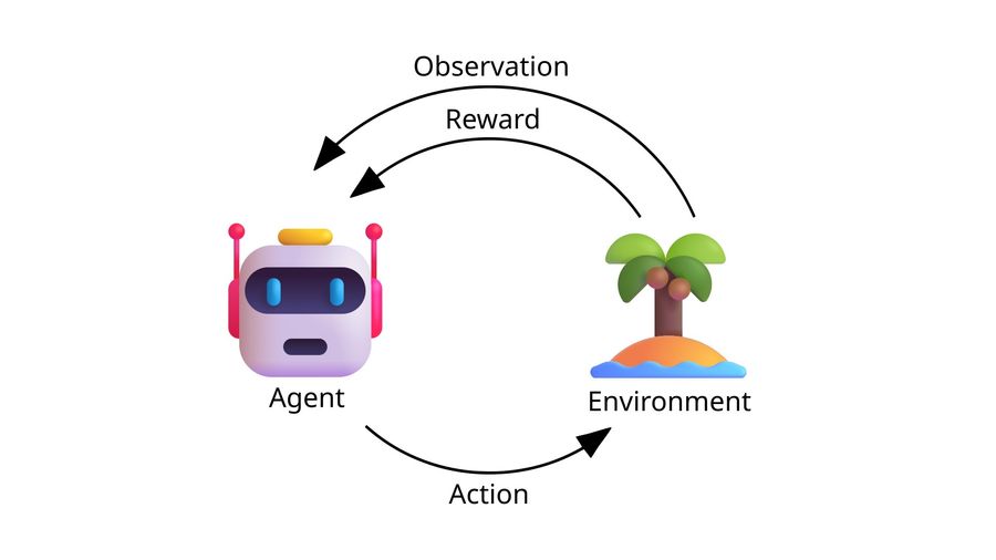
Before we dive into the custom reinforcement learning environment, I want to provide you with a basic understanding of reinforcement learning. Reinforcement learning uses a feedback-response-loop for training. A diagram of the feedback-response-loop is displayed below. The Environment defines the problem that the AI is trying to solve. The environment generates an Observation (or “state”) which is a snapshot of the current state of the environment and a Reward which represents the quality of the selected actions by the AI. The observation can be handcrafted data, images or vectors. Both observation and reward are then sent to the Agent. The agent is a program, that interacts with the environment by using a specific reinforcement learning Model to select one Action from all possible actions (also called Action Space). The selected action then changes the environment, which closes the feedback-response-loop and initiates a new Step in the training. The feedback-response-loop continues until a specified end-condition is met.

Reinforcement learning is a framework for solving control tasks (also called decision problems) by building agents that learn from the environment by interacting with it through trial and error and receiving rewards (positive or negative) as unique feedback.

If you want to learn more about reinforcement learning models and its correct implementation, I highly recommend this resource.

Basic Structure Of An Environment

Every gym environment has the same basic outline.

import gym

class CustomEnvironment(gym.Env):
    metadata = {'render.modes': ['human']}

    def __init__(self) -> None:
        super(CustomEnvironment, self).__init__()
        self.reward_range = ...
        self.action_space = ...
        self.observation_space = ...
        ...
        self.reset()

    def reset(self, seed=None):
        ...
        return observation

    def step(self, action):
        ...
        return observation, reward, done, info
    
    def render(self, mode='human', close=False) -> None:
        ...

`init()`

Handles the initial setup of the environment. In the initial setup of our environment we need to define 3 variables:

reward_range = (-inf, inf): Defines the minimal and maximal reward that the agent can achieve.
action_space: Space[ActType] : Defines what actions the agent can take.
observation_space: Space[ObsType]: Defines all possible stages the environment can be in.

`reset()`

Rests the environment to its initial state. To create reproducible environments you can set the seed parameter to a specific number. The reset() function returns an observation which is a value within the observation_space.

`step()`

Calculates the next increment of the environment based on the selected action. After calculating the new state of the environment the following values are returned:

observation (object): A new state of the environment, withing the bounds of the defined observation_space.
reward (float): Defines how good the selected actions of the agent were.
done (bool): Indicates, if a simulation episode has ended.
info (dict): Allows you to pass additional diagnostic information (helpful for debugging, learning, and logging)
Optional:
- terminated (bool) : Indicates if a terminal condition is met.
  Further step calls would return undefined.
- truncated (bool): Indicates if a truncation condition is met. Typically, it is used for a time-limit, but it can also be used to indicate that an agent is physically going out of bounds.

`render()`

Allows you to define how the environment is displayed. This can be anything from text prompts to 2D or 3D graphics.

Spaces

Spaces define the range of values that are allowed in an action or an observation

Box: describes an n-dimensional continuous space. It’s a bounded space where we can define the upper and lower limits of this space. Every value within the bounds can appear.
- Identical bound for each dimension:
```
Box(low=-1.0, high=2.0, shape=(3, 4), dtype=np.float32)
# Box(3, 4)
```
- Independent bound for each dimension:
```
Box(low=np.array([-1.0, -2.0]), high=np.array([2.0, 4.0]), dtype=np.float32)
# Box(2,)
```
Discrete: Describes a space consisting of finitely many elements. This class represents a finite subset of integers, more specifically a set of the form
$\{a, a+1, …, a+n-1\}$ .
```
Discrete(2)            
# {0, 1}

Discrete(3, start=-1)  
# {-1, 0, 1}
```
Dict: represents a dictionary of simple spaces.
Tuple: represents a tuple of simple spaces.

MultiBinary: creates a n-shape binary space.

MultiBinary(5)
# array([0, 1, 0, 1, 0], dtype=int8)
observation_space = MultiBinary([3, 2])
# array([[0, 0], [0, 1], [1, 1]], dtype=int8)

MultiDiscrete: consists of a list of Discrete action spaces. Each Discrete space can have a different number of actions in each element.
```
MultiDiscrete([ 5, 2, 2 ])
# array([3, 1, 0])
```
There are a few more unique spaces like Graph, Squence, or Text, which you can read more about here

Not every RL model supports every space we described. If you are using stable-baselines3 the following table allows you to choose a RL model based on the action spaces you used:

Name	`Box`	`Discrete`	`MultiDiscrete`	`MultiBinary`	Multi Processing
ARS 1	✔️	✔️	❌	❌	✔️
A2C	✔️	✔️	✔️	✔️	✔️
DDPG	✔️	❌	❌	❌	✔️
DQN	❌	✔️	❌	❌	✔️
HER	✔️	✔️	❌	❌	❌
PPO	✔️	✔️	✔️	✔️	✔️
QR-DQN 1	❌	️ ✔️	❌	❌	✔️
RecurrentPPO 1	✔️	✔️	✔️	✔️	✔️
SAC	✔️	❌	❌	❌	✔️
TD3	✔️	❌	❌	❌	✔️
TQC 1	✔️	❌	❌	❌	✔️
TRPO 1	✔️	✔️	✔️	✔️	✔️
Maskable PPO 1	❌	✔️	✔️	✔️	✔️

Tuple observation spaces are not supported by any environment.
Dict observation spaces are supported by any environment.

Wrappers

Wrappers allow you to transform existing environments without having to alter the used environment itself. Wrappers can also be chained to combine their effects.

import gym
from gym.wrappers import RescaleAction

base_env = gym.make("BipedalWalker-v3")
# base_env.action_space: Box([-1. -1. -1. -1.], [1. 1. 1. 1.], (4,), float32)
wrapped_env = RescaleAction(base_env, min_action=0, max_action=1)
# wrapped_env.action_space: Box([0. 0. 0. 0.], [1. 1. 1. 1.], (4,), float32)

Here you can read more about the different wrappers available.

Example Environment

To provide you with a more specific example, I have broken down the environment we created in our prove of concept. The idea of this environment is to imitate a simple purchase behavior of a consumer based on price and expiration date.

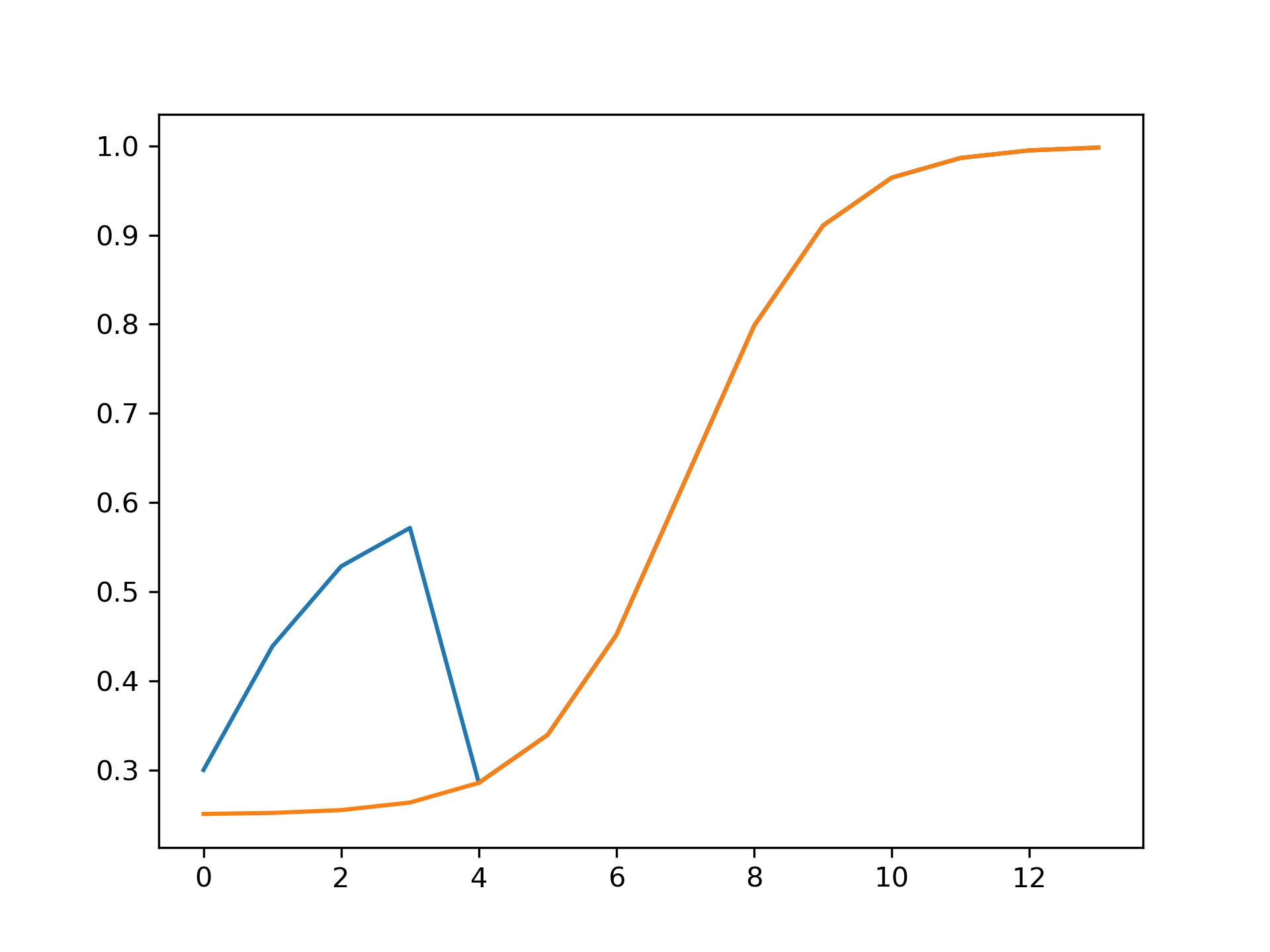
We modeled the consumer behavior based on recent studies and found that the likeness to buy, based on the expiration date, declines in a shape of a sigmoid function. We additionally found that around 50% - 60% of people would buy nearly expiring discounted products if they had a discount. The following diagram illustrates the consumer behavior without discount in orange and with a 15% discount in blue.

import numpy as np
import math

def customSigmoid(x, a, b, c, d):
    """ General sigmoid function
    a adjusts amplitude
    b adjusts y offset
    c adjusts x offset
    d adjusts slope """
    return ((a-b) / (1 + np.exp(x-(c/2))**d)) + b

def likeness_to_buy(x, discount_days, total_days, discount):
  return max(customSigmoid(x, 1, 0.25, total_days, -1), 
             customSigmoid(x, 4*discount, 0, 0, -1) 
             if x <= discount_days else 0)

Next, we created the __init__(). To simplify things, our shelf only has items that cost the same amount of money. We then create a random number of products with different expiration dates. Then we give our agent the possibility to choose the discount percentage, that every nearly expiring product gets. We give one discount for all nearly expiring products, because our hypothesis was, that multiple discounts for each expiration date would confuse consumers.

def __init__(self) -> None:
    super(PricelessEnvironment, self).__init__()

    self.reward_range = (0, MAX_REVENUE)

    # Actions: define the discount of nearly expired products
    self.action_space = spaces.Box(
        low=0, high=MAX_DISCOUNT, shape=(1,), dtype=np.float32)

    # Observation: ShelfLive, where the index is the shelf live in days and revenue
    self.observation_space = spaces.Dict({
        "ShelfLife": spaces.Box(
            low=0,
            high=INITIAL_NUMBER_OF_PRODUCTS,
            shape=(PRODUCT_LIVE_TIME,),
            dtype=int
        ),
        "Revenue": spaces.Discrete(MAX_REVENUE)
    })

    self.reset()

At the end of our __init__() function we call the reset() function to initialize all variables. In our case we tracked the following variables to train our model:

def reset(self):
    self.done = False
    self.current_step = 0
    self.reward = 0
    self.sold_products = 0
    self.expired_products = 0

    self.revenue = 0
    self.discount = 0
    # generate a random set of expiring products
    self.shelf_life = np.zeros(shape=(PRODUCT_LIVE_TIME,), dtype=int)
    for _ in range(INITIAL_NUMBER_OF_PRODUCTS):
        self.shelf_life[random.randint(PRICE_REDUCTION_DAYS, len(self.shelf_life)-1)] += 1

    return self._next_observation()

The function _next_observation() is called, whenever the next step of the simulation should be calculated. In an environment, this happens at two stages, when you reset the environment (reset()) and when you calculate the next step (step()). In our example, we first calculate the consumer behavior and then remove the expired products.

def _next_observation(self) -> dict[str, Any]:
    # remove bought items
    self._consumerSimulation()

    # remove expired items
    for index in range(self.current_step):
        if (index > PRODUCT_LIVE_TIME): continue
        self.expired_products += int(self.shelf_life[index])
        self.shelf_life[index] = 0

    # Update the expiration dates of the remaining stock
    obs = {
        "ShelfLife": self.shelf_life,
        "Revenue": self.revenue
    }
    return obs

The consumer behavior of one consumer is calculated by randomly selecting three items. The consumer then calculates the likeness to buy the item based on its expiration date and available discount. If the likeness to buy is great enough, the item is bought.

def _consumerSimulation(self) -> None:
    if self.current_step <= 1: return
    for _ in range(NUM_OF_CONSUMERS):
        self._consumerAction()

def _consumerAction(self) -> None:
    if (self.shelf_life.sum() == 0): return
    
    selected_prods_shelf_life = [index for index, elem in enumerate(self.shelf_life) if elem != 0]
    # Consumer picks up three random items
    picked_shelf_life = random.choices(
        selected_prods_shelf_life, 
        [self.shelf_life[items] / self.shelf_life.sum() for items in selected_prods_shelf_life], 
        k=NUM_OF_INSPECTED_ITEMS_BY_CONSUMER)
    
    # Consumer calculates likeness to buy
    for shelf_life in picked_shelf_life:
        if random.random() <= likeness_to_buy(shelf_life, discount_days=PRICE_REDUCTION_DAYS, total_days=PRODUCT_LIVE_TIME, discount=self.discount):
            self.shelf_life[shelf_life] -= 1
            self.sold_products += 1 
            if shelf_life <= PRICE_REDUCTION_DAYS:
                self.revenue += PRICE_RECOMMENDATION * (1 - self.discount)
            else:
                self.revenue += PRICE_RECOMMENDATION

In our step() function, we implement the simulation loop. First, the AI is performing its action, which is defined in the _take_action() function. Then based on the chosen action a new observation and a new reward is generated. Last, the end condition of the simulation is checked.

def step(self, action):
    self.current_step += 1
    self._take_action(action)
    
    prev_revenue = self.revenue
    prev_expired_products = self.expired_products
    obs = self._next_observation()

    self.reward += self.revenue - prev_revenue - ((self.expired_products - prev_expired_products) * PRICE_RECOMMENDATION * (1 - self.discount))
    if self.shelf_life.sum() == 0:
        self.done = True

    return obs, self.reward, self.done, {}

In our case, the _take_action() function just changes the discount, but you could implement sophisticated action analysis. We could, for example, track the number of discount changes and reduce the reward if the discount is changed too often.

def _take_action(self, action):
    self.discount = float(action)

Lastly, the render() method displays the current state of the environment of a simulation. The environment can be rendered in many ways, like 2D graphics, vectors, or just text. For our project, a text output is sufficient.

def render(self, mode='human', close=False) -> None:
    if mode == 'human':
        print(f'Step: {self.current_step}')
        print(f'Avg price of sold products: {0 if self.sold_products == 0 else self.revenue / self.sold_products}')
        print(f'Revenue in cents: {self.revenue/100}')
        print(f'Sold Products: {self.sold_products}')
        print(f'Expired Products: {self.expired_products}')
        print(f'Remaining Products: {self.shelf_life.sum()}')
        print(f'Current Discounted Price: {PRICE_RECOMMENDATION * (1 - self.discount)}')
        print("=======================================================")

🧪Test Your Environment

Because we cannot directly see what the reinforcement learning agent is learning, we need to make sure, that our environment is behaving as expected beforehand. Without this crucial step, the results of the RL agent are mediocre at best.

Checking API-Conformity

Before we use the environment in any kind of way, we need to make sure, the environment API is correct to allow the RL agent to communicate with the environment. A simple API tester is already provided by the gym library and used on your environment with the following code.

from gym.utils.env_checker import check_env
check_env(env)

Testing With Possible Actions

If the API of our environment is correctly functioning, we can further test our environment with either deliberately choosing certain actions or by randomly selecting actions from the action space.

In our example below, we chose the second approach to test the correctness of your environment. We additionally render each observation with the env.render() function and render the final result after the simulation is done.

obs = env.reset()
while True:
    action = env.action_space.sample()
    obs, reward, done, info = env.step(action)
    env.render()
    if done:
        print("{} products expired".format(env.expired_products))
        print("Generated revenue {}".format(env.revenue))
env.close()

💪Train Your Model

After creating and testing our environment, we can train our RL model in our environment. As stated earlier, if you want to learn more about RL models, I highly recommend this resource.

from stable_baselines3 import PPO

env = PricelessEnvironment()

model = PPO("MultiInputPolicy", env, verbose=1)
model.learn(total_timesteps=3000)
model.save("./priceless_rl")

🏁 Compare Our RL Agent

Lastly, we compare our trained reinforcement learning agent with the simple strategy of not giving a discount at all. To achieve this, we load our trained model and create a dummy model that just returns a constant action. In our example, the constant action a discount of 0%. Then we define the run_with_model() function, that chooses an action as long as the simulation is not done. To ensure accuracy in our comparison results, we take the average comparison results in average_model_results().

from stable_baselines3 import PPO

ppo = PPO.load("./priceless_rl", env=env)

class DummyModel:
    def predict(self, obs):
        return 0, None

dummy = DummyModel()

def run_with_model(model):
    obs = env.reset()
    while True:
        action, _states = model.predict(obs)
        obs, reward, done, info = env.step(action)
        env.render()
        if done:
            return env.expired_products, env.revenue

def average_model_results(model):
    EXECUTIONS_TO_RUN = 100
    expireds, revenues = zip(*[run_with_model(model) for i in range(EXECUTIONS_TO_RUN)])
    def mean(lst):
        return sum(lst) / len(lst)
    return mean(expireds), mean(revenues)


ppo_expired, ppo_revenue = average_model_results(ppo)
dummy_expired, dummy_revenue = average_model_results(dummy)

print(str(dummy_expired - ppo_expired) + " fewer products expired with RL")
print(str(ppo_revenue - dummy_revenue) + " more profit with RL")

Our final result after the short development of our proof of concept achieved a 29% decrease in food waste and a 1.7% increase in revenue. This is a good result, but can’t be simply applied to the real world. To apply it to the real world, we have to develop a more realistic environment.